managerial economics questions

Economics Homework Help

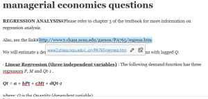
REGRESSION ANALYSISPlease refer to chapter 3 of the textbook for more information on regression analysis.

Also, see the linkhttp://www2.chass.ncsu.edu/garson/PA765/regress.htm

We will estimate a demand function using linear and log-linear regressions with lagged Q.

· Linear Regression (three independent variables) : The following demand function has three regressors P, M and Qt-1 .

Qt = a + bPt + cMt + dQt-1

where: Q is the Quantity (dependent variable)

P is the Price

M is the Income

Qt-1 is the lagged Q

t is the time period

· Input or copy the data on an EXCEL sheet, clearly specifying the dependent Y variable to be the quantity (Qt) (highlight its column), and the independent X variables to be the price (Pt), income (Mt) and the lagged Qt-1 or as the situation warrants.. Here we have three regressors: (Pt), income (Mt) and the lagged Qt-1 (highlight all of them at the same time).

· To enter values for the lagged Qt-1, you may copy the whole data under Qt and paste it in a new column added to the given sheet under the lagged Qt-1. Pasting should start such that the first observation under Qt will be the first observation under the lagged Qt-1 starting with the second row

· Click on Excel icon on top left, Excel Options at the bottom of pop up menu,  Add-ins in the left hand column, then Analysis Toolpak, then hit ok.

· if it does not come up, then hit go and make sure that Analysis Toolpak is checked.

· then under Data, Data analysis, Regression, ok.

· If you have Analysis Toopak in your computer, then the road to regression is shorter. Click on Excel icon, Data, Data Analysis in the up far right  then Regression.

· Go to TOOLS menu and click DATA ANALYSIS. Pick up REGRESSION from the ANALYSIS TOOLS presented in the pop up menu and click OK.

· First highlight the dependent variable (Qt) cell range from the spreadsheet starting from the second row (skip the row with the empty cell), and click OK on the REGRESSION pop up menu to insert the selected data range in the Input Y range box. Similarly select the relevant data range for all the independent variables together including lagged Q and insert the selected data range in the Input X range box. Double check your cell ranges.

· Click on “LABEL” to include the symbols or names of variables in the regression output.

· In the OUTPUT OPTIONS, click New Worksheet Ply and say OK. The Regression output will be available to you on a newly created worksheet.

How to add DATA ANALYSIS to your TOOLS menu?

· If the TOOLS menu in your computer does not have DATA ANALYSIS, you can add it by doing the following.

· Open TOOLS

· Click on ADD-INS

· Include ANALYSIS TOOLPACK from the pop up menu dialog box and click OK.

· Go back to TOOLS and you will find DATA ANALYSIS at the bottom of the menu.

The Questions required for the homework assignment are listed

Below: Homework assignment: Questions

QUESTION 1:

Copy the database below into an excel sheet.

Run QX on the four regressors: PX, M, PY and lagged Qx.

Write down the estimated linear demand equation with t-statistics under the estimated coefficients as done above. In addition, write down the R-square and explain what it means. Explain the statistical significance of the t-statistics for each regressor. Significance of T-statistics is usually given by the P-values in the regression output. We will not use it in here because we have a small sample which will bias the P-values. There are three levels of significance: 1%, 5% and 10% represented by ***, ** and *, respectively. Do not use the computed P-values of this small sample regression. Instead, use the following conventional t-statistics significance ranges used for large data:1.63 <t < 1.96 (10%); 1.96 < t < 2.54 (5%); and t > 2.54 (1%). This means in your regression output, look at the t-statistics column for each regressor. Then place the value of that computed t-statistic in one of the above ranges. The P-values given in the regression output are sensitive to sample size and are not accurate.

QUESTION 2

Check the signs of the estimated coefficients. Do the signs follow the theory as expected? Examine the sign for each regressor and point out what they mean.

QUESTION 3:

Calculate the short-run and long-run price and income elasticities of demand for good X using the averages for the quantity, price and income? Based on the income elasticity, what type is good X?

Short Run P elasticity for a linear Eq. = [slope of price]*(Average Price/Average quantity)

Long Run P elasticity for a linear Eq. = (SR P elasticity) /(1- slope of lagged Q)

or = [slope of price / (1- slope of the lagged variable)]*(Average Price/Average quantity).

They are the same.

Average = sum/n, skipping first row.

The short-run and long run income elasticities are calculated the same way. Here the slope is for income and the average for income (see page 31 or the solved regression on pp 32-33). What type of good is X with respect to income elasticities?

Short Run Income elasticity for a linear Eq. = [slope of Income]*(Average Income/Average quantity)

Long Run Income elasticity for a linear Eq. = (SR Income elasticity)/(1- slope of lagged Q)

QUESTION 4:

Calculate the short-run and long-run cross price elasticities with respect to Py (see p. 28 and p. 30 in the notes). What type of goods are X and Y with respect to these elasticities?

QUESTION 5

Can you think of another independent variable that you may add to the above equation? What will the sign of this variable be? Specify the name of this variable. Do not include Weather in this equation.

QUESTION 6

Is this a supply or demand equation? Why? Forget about signs. Look for other clues in the equation.